Charge flipping
with neutron TOF single crystal data
In this exercise you will use GSAS-II to solve the structure of rubrene (C42H28) from single crystal neutron data via charge flipping. Rubrene is of interest as a molecular semiconductor. It crystallizes in the space group Cmca with the lattice parameters a=26.798Å, b=7.1618Å, c=14.1942Å, Z=4. Thus, the molecule is sited on a special position with 2/m symmetry. If you have not done so already, start GSAS-II.
Step 1. Set the phase information
To begin this tutorial, do Data/Add new phase in the main GSAS-II data tree menu. A popup window will appear asking for a phase name; I used rubrene. The General tab for this phase will be shown
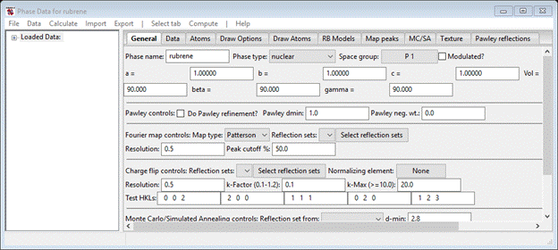
Enter the space group (C m c a – don’t forget the spaces) and press Enter. A popup with Space group information will appear
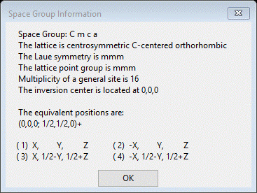
Press OK; the General tab will be repainted with defaults for the orthorhombic lattice parameters. Enter 26.798 for a, 7.1618 for b and 14.1942 for c. Press Enter, the unit cell volume (2724.178) will be updated.
Step 2. Import the data
The rubrene data were collected on the TOPAZ instrument at the SNS Facility, Oak Ridge National Laboratory with 23 different crystal orientations; the local instrument data processing software has applied corrections and combined them into a single multicolumn hkl file. To import this do Import/Structure Factor/from Neutron TOF HKL F2 file; a directory dialog box will appear. Go to the directory TOF Charge Flipping/data and select the file ruberene_orthoC.hkl (double click the name or press the Open button after selecting it). A popup box will appear.
Press Yes; another popup will appear offering you the chance to change the name. Press OK, a new popup appears.

Here you select the phase the data belongs to. There is only rubrene so select it and press OK. The bottom of the data tree is shown, a small data window and the plot shows the l=0 slice of the last reflection set loaded (HKLF rubrene_orthoC.hkl_22).
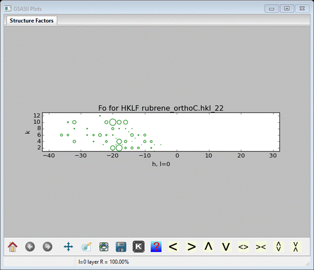
The K box control allows you to select other zones & layers to view. The drawing geometry is strictly square (i.e. not in reciprocal space units). If you do Commands/Plot 3D HKLs, a 3D plot of reciprocal space is shown

The size of the green boxes is proportional to the structure factors; the save as/key pulldown will give you other viewing options. Here is a good place to save the GSAS-II project for rubrene. Do File/Save project from the main GSAS-II data tree window; a file dialog box will appear. Enter a file name (I used rubrene – no extension).
Step 3. Setup for charge flipping
We have two tasks here. One is to select the reflection sets to be used in the calculations and the other is to set some controls. To begin select the rubrene phase entry in the GSAS-II data tree; the General tab will appear in the Phase Data for rubrene window
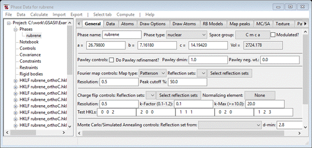
In the Charge flip controls (about center of the page) press the Select reflection sets button; a Use data popup will appear. You will want to use all the HKLF data sets; press Set All and press OK. The General tab will be refreshed. GSAS-II will use all the data to build a reflection set for charge flipping. For duplicate hkls the last one encountered will be used. Since atoms are essentially point scatterers for neutrons, a charge flip map has very sharp peaks so a better choice for the k-factor (charge flip level) might be 0.5, the k-max should be larger (say 50) and the map Resolution should be smaller (say 0.4). Set these three values. In the Fourier map controls, set Peak cutoff % to 20; this sets the lower limit of the peak search in the charge flip map. When done the General tab should look like

Step 4. Charge flipping
We are now ready for charge flipping. In the General tab menu do Compute/Charge flipping; a Charge flipping progress bar will appear showing the residual and cycle count for the charge flipping calculation. In this case the residual quickly drops to ~38% and stays there. Press Cancel to stop the calculation; some information will be printed on the console and after a pause the Phase Data window will show Map Peaks and the plot window will show a drawing of the obtained structure.
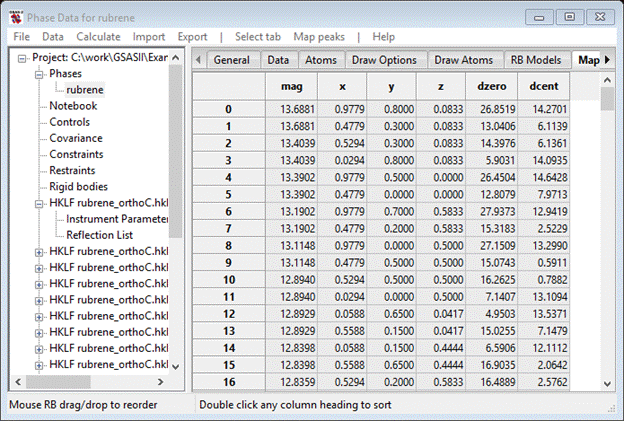
If you scroll down the Map peak list you will find some with negative magnitudes at the end of the list. GSAS-II searches the map for both positive and negative peaks; the former are C-atoms and the latter are H-atoms.
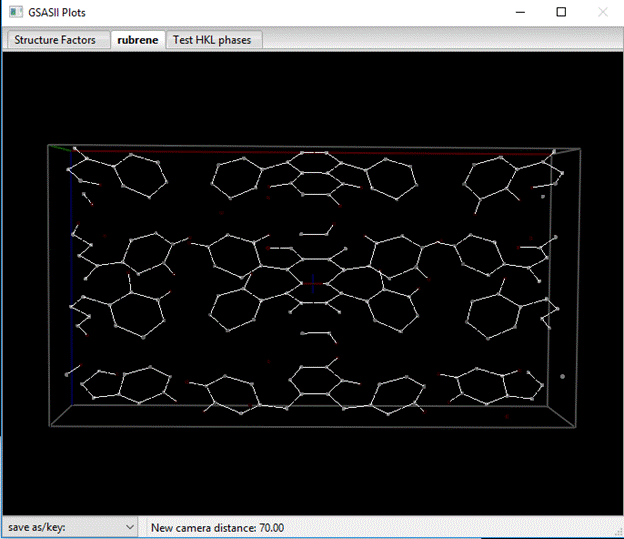
The plot (which I’ve rotated around a bit) shows white spots for the positive peaks and red ones for the negative ones; bonds are white lines. Your solution may show a problem with the charge flip solution. While the charge flipping run has clearly found all the C-atoms and some of the H-atoms, the molecule may be incorrectly placed in the unit cell (the multicolored cross should be in the middle of the C-C bond at the center of the molecule). To fix this you could simply repeat the charge flipping run and hope it puts the molecule in the right place. GSAS-II uses an algorithm based on how structure factor phases are related for a given space group to reposition the solution; it sometimes fails if the phase set isn’t perfect. Or you can “roll” the map right/left/up/down (R/L/U/D keys) to put the solution where you want. Notice that as the map is rolled, the Map peak positions are shifted to match the change in positions.
By carefully looking at the map, you can see the 4-ring tetracene (naphthacene) core of the molecule with four phenyl groups attached to both sides on the center two rings. The unique part consists of 1/4th of this group (i.e. half of one side of the tetracene and one phenyl); one C-atom sits on a 2-fold and the rest are in general positions. The molecule extends into the neighboring unit cell so you don’t see the whole thing as one group but has two bits on either side.
Step 5. Peak selection
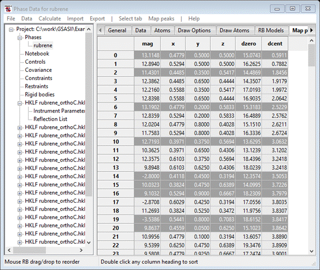
GSAS-II provides several ways of selecting peak positions from a charge flipping map. One way is to pick them directly from the drawing. Place the cursor on one peak and do a Shift left mouse button; it will be highlighted on the list and it will turn green on the plot. Do a Shift right mouse button on the remaining peaks you want to pick. All will turn green (you may have to wiggle the plot a bit with the mouse to make them show) and all will be highlighted in the list. Alternatively, you can select the entire list of peaks (double click on upper left empty box of the table), then do Map peaks/Unique peaks. Better still you can sort the peaks by one of the column headings and then do Map peaks/Unique peaks. I’ve chosen to sort the peaks on dcent (distance from center of the cell) beforehand. After a pause while it sorts out the unique peaks, it will highlight them in the table and display the picked ones in green on the plot. In this case they will probably be scattered about the unit cell and not make a continuous molecule, but they are largely clustered around the unit cell center. My plot looked like this when I was done.
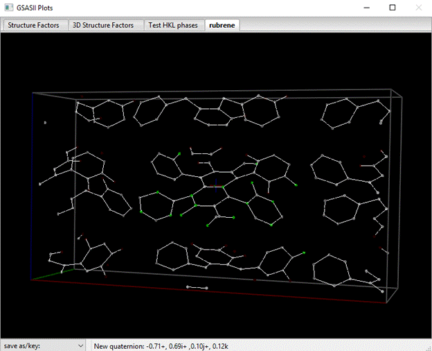
The list has them highlighted (the rest are lower down in my list; all 18 atoms were found in this charge flipping result)
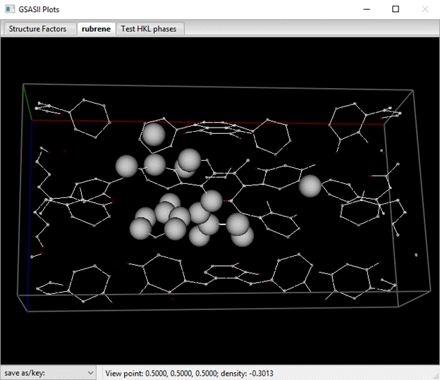
To add them to the Atom list do Map peaks/Move peaks; the drawing will show white balls for them.
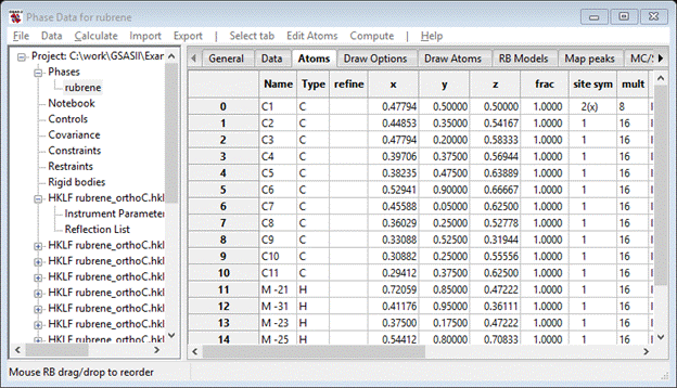
The atom list will give the magnitudes as ‘M’ names; I found all 11 C-atoms and 7 H-atoms that were expected.

Step 6. Atom identification
You can reorder the atoms in the list; do an Alt select for the atom row you want to move. Then do an Alt select on the row where you want the moved atom to precede it. This way you can put the C-atoms first and the H-atoms last in the list instead of mixed up as in the above list. Next select all the positive M peaks (pick the top one and then Shift pick the last one). Do Edit Atoms/On selected atoms/Modify parameters from the Atoms menu; a popup will appear. Pick Type and press OK; a Periodic Table will appear. Select C from the C-atom pulldown. All the C-atom names and types will change and the plot will show dark gray spheres for the C-atoms. You should also move the C-atom with 2(x) site symmetry to the top of the list (if it isn’t there already).
Do the same with the remaining negative M atoms – make them H atoms. The drawing shows molecular fragments scattered about the unit cell; you’d like to unify them into a single molecule. Select the C-atom with 2(x) site symmetry (although any would do). Do Edit Atoms/Assemble molecule from the Atoms menu; a popup will appear offering choices for Bond radii (& Angle radii – ignored here). Press Ok; the Atom table will be revised and the plot will show an assembled molecule.
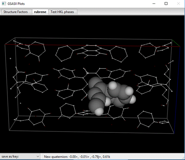
The molecule building has scrambled the order of the atoms; they were located in order as the molecule was built.
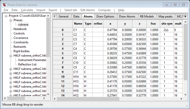
You can reorder them to put the H-atoms at the end of the list (if they weren’t there already). Then select all of them and then do Edit Atoms/On Selected atoms…/Modify parameters. Pick Name from the pulldown and press OK. You are asked if you really want to do this, press Yes. The atoms are then renamed in numeric order.
Step 7. Refinement
Since the structure is complete, we can do the full refinement. Select the Controls item from the GSAS-II data tree. Unset the Refine HKLF as F^2 box and enter 3.0 for Min obs/sig. This makes the least squares refine on Fo with 3σ cutoff on Fo. From the main GSAS-II data tree menu do Calculate/Refine; this will do the 1st least squares refinement varying only the data set scale factors. A progress bar popup will appear showing the residuals as the refinement proceeds. When done, a small popup will appear with the final residual; press OK to accept it. The final Rw is about 47% Go to the Atoms tab for the rubrene phase, double click the refine column heading; a popup box will appear. Select both X - coordinates and U – thermal parameters and press OK. The atom table will show refine flags for each atom.
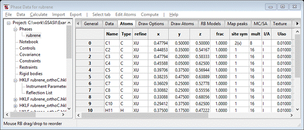
Then repeat the Calculate/Refine (twice)command in the main menu. The final residual will be much better Rw ~10%. Next, convert all the atoms from isotropic thermal parameters to anisotropic ones. Double click the I/A column heading and select Anisotropic and press OK. Then repeat Calculate/Refine (perhaps twice); the final Rw ~5.9% which is quite nice.
Step 8. Further work
Since this is TOF neutron single crystal diffraction, a relatively large crystal was used and the neutron wavelength covered a fairly wide range of values. Hence, it is likely that the strong reflection intensities suffered from some level of extinction. To find these parameters select the Data tab in the Phase Data window; all that will show is a list of a data set names with the 1st one highlighted; the window will look something like

The Scale factors is selected for refinement by default (box checked). Here you want to select Primary for the Extinction type (later you can try the other models) for the 1st data set. The window will be repainted with a new line in the data display. Select the Ep check box so it will be refined. To set all the rest do Edit Phase/Copy FlagsA popup will appear giving the list of data sets; press the Set All button and then OK. You could then do Calculate/Refine but it might be better to constrain all the Ep values to be the same. To do this select Constraints from the GSASII data tree. A blank window with tabs will appear.
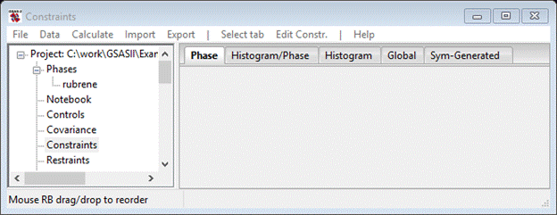
Select the Histogram/Phase constraints tab; the window is still blank but that tab is now highlighted. Next do Edit Constr./Add equivalence; a popup will appear asking for a parameter name to be constrained.

Select 0:0:Ep, that is the primary extinction parameter for the 1st dataset and the rubrene phase. Press OK.
The popup is replaced with a new list of all compatible parameters that 0:0:Ep is to be made equivalent to. Scroll down and find 0:all:Ep and pick that and press OK; the Constraint window will change to
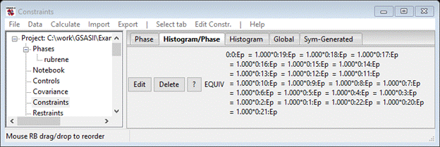
This shows the constraint making Ep for all 23 data sets equivalent to a single variable. Do Calculate/Refine; my Rw was 5.474% only a slight improvement. You may wish to try the other extinction models. Do remember to delete the unused constraint before adding a new one for the different extinction parameter. Finally you can draw the molecule; go to Atoms and do Edit Atoms/Reload draw atoms. That will put the newest atom parameters into the Draw Atoms table. Select Draw Atoms. Select the Style column heading; a popup will appear
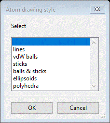
Notice the first line is blank, if you select that all the atoms will vanish! Select ellipsoids and press OK. I also set the ellipsoid probability to 99% (slider on the Draw Options tab). The plot will change, but it is pretty cluttered.
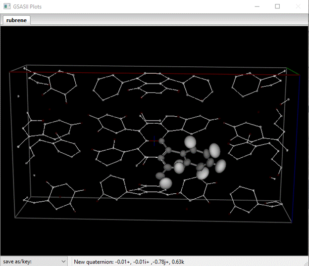
You can remove the Map peaks atoms; go to the Map peaks tab and do Map peaks/clear peaks from the menu. The list will be erased and the plot will just show the molecule. You can also remove the unit cell edges, go to Draw Options and uncheck the Show unit cell? box. Finally, you can remove the charge flipping map; go to General and do Compute/Clear map. That deletes the scattering density map and the drawing will be free of any clutter.

Remember that this is only 1/4th of the molecule, we’d like to see the whole thing. First go to the Atoms tab and select the C-atom that is in a special position 2(x). The do Compute/Show Distances & Angles and respond OK to the popup. The important result is on the console
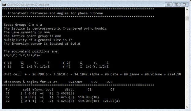
This gives the bond distances and angles about the C(1) atom. Particularly note the cell+(sym. Op.) information; we will use this to build the drawing. Go to the Draw Atoms tab and select all the atoms (double click on the upper left box). You should see all atoms selected

Then do Edit Figure/Add atoms; a popup will appear
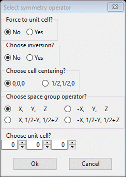
Based on the 1st entry in the bond distance table ‘[1 0 0] +( 2)’, select the controls for the 2nd operator and increment the 1st unit cell

Press OK. The plot now shows ½ the molecule.
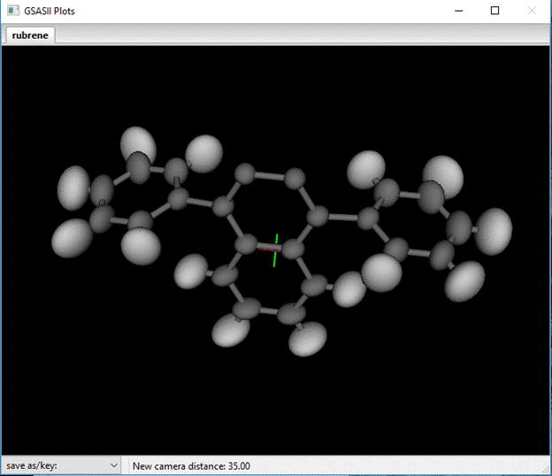
Next select all the Draw atoms again and do Edit Figure/Add atoms; the selection popup will appear. This time use the other nonidentity entry in the bond distance table ‘[0 1 1] + (-2)’. The ‘-2’ indicates both the inversion and the 2nd operator need to be applied; check both and increment the 2nd and 3rd unit cell entries.
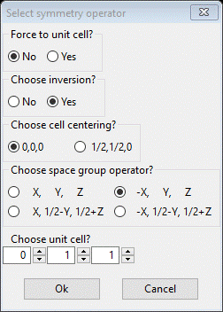
Press OK; the entire molecule is drawn.

Looks really nice. This ends the tutorial. You can save the project if you wish. All the changes (i.e deleting Map peaks & clearing the map) will be saved.